Skip to content

3. Markov Chain & Markov Sampling

1. Markov chains โ€‹

(1) State transition probability โ€‹

Markov property The next state depends only on the current state, not on the past states.

Let (Xt)tโ‰ฅ0 be a discrete-time Markov chain on a state space S={a1,a2,โ€ฆ}. It satisfies the Markov property:

(1.1.1)Pr(Xt+1=jโˆฃXt=i,Xtโˆ’1,โ€ฆ,X0)=Pr(Xt+1=jโˆฃXt=i).

Thus, conditional on the current state, the next state is independent of the earlier history. For a time-homogeneous chain, this conditional probability does not depend on t. Define the one-step transition probabilities and transition matrix by

(1.1.2)Pij=Pr(Xt+1=ajโˆฃXt=ai),P=(Pij).

This note uses the row-vector convention: row i gives the probabilities of moving from ai to the possible next states. Therefore,

(1.1.3)Pijโ‰ฅ0,โˆ‘jPij=1.

For example, a finite-state transition diagram may be represented by the matrix P, whose entry Pij is the label on the directed edge aiโ†’aj.

(2) Multi-step transition probabilities โ€‹

We define ==the n-step transition probability== as :

(1.2.1)pij(n)=Pr(Xt+n=ajโˆฃXt=ai).

Let P(n)=(pij(n)). The Chapman-Kolmogorov equation (C-K equation) is defined as the transition probability relation on state transition i-> k -> j summed on every possible intermediate states k :

(1.2.2)pij(m+n)=โˆ‘kโˆˆSpik(m)pkj(n).

pij(m+n)=Pr(Xt+m+n=ajโˆฃXt=ai) is the probability that the chain reaches state aj after m+n steps, given that it starts at ai.

In particular, for a time-homogeneous chain, it satisfies the Markov condition, the relation of :

(1.2.3)P(n)=Pn,pij(n)=โˆ‘kโˆˆSPikpkj(nโˆ’1).

Equivalently, expanding over all intermediate states gives :

(1.2.4)pij(n)=โˆ‘k1,โ€ฆ,knโˆ’1โˆˆSPik1Pk1k2โ‹ฏPknโˆ’1j.

If the initial distribution is the row vector ฮผ0, then the distribution after n steps is

(1.2.5)ฮผn=ฮผ0Pn.

(3) Limiting distribution โ€‹

A distribution ฯ€ is a limiting distribution of state transformmatrix P when

(1.3.1)limnโ†’โˆžฮผ0Pn=ฯ€

for every initial distribution ฮผ0. For a finite Markov chain, irreducibility and aperiodicity are sufficient for a unique limiting distribution. More generally, suitable recurrence conditions are also required on an infinite state space.

2. Stationary distributions and detailed balance โ€‹

(1) Stationary distribution โ€‹

A probability distribution ฯ€=(ฯ€1,ฯ€2,โ€ฆ) is stationary for P if :

(2.1.1)ฯ€P=ฯ€,โˆ‘iฯ€i=1,ฯ€iโ‰ฅ0.

Component wise, the stationarity condition is :

(2.1.2)ฯ€j=โˆ‘iฯ€iPij.

If a chain is initialized from ฯ€, it remains distributed as ฯ€ after every transition. In MCMC, ฯ€ is the target distribution; after convergence, the chain states can be used as dependent samples from ฯ€.

(2) Detailed balance โ€‹

To make sure a distribution is a stationary distribution, A convenient sufficient condition for stationarity is detailed balance (or reversibility) :

(2.2.1)ฯ€iPij=ฯ€jPjifor allย i,j.

Indeed, summing over i and using โˆ‘iPji=1 gives

(2.2.2)โˆ‘iฯ€iPij=โˆ‘iฯ€jPji=ฯ€j.

Detailed balance is sufficient, but not necessary, for ฯ€ to be stationary.

3. Markov Chain Monte Carlo (MCMC) โ€‹

MCMC constructs a Markov chain whose stationary distribution is a chosen target density or mass function ฯ€(x). It is especially useful when direct independent sampling from ฯ€ is difficult, while evaluating ฯ€(x) up to a normalizing constant is feasible.

Starting from an arbitrary initial state X0=x0, run a transition kernel that leaves ฯ€ invariant. After a suitable burn-in period, retain states Xt as samples. Because consecutive states are correlated, effective sample size is generally smaller than the number of retained iterations.

Target density need not be normalized In Metropolis-Hastings, only ratios such as ฯ€(y)/ฯ€(x) are used. Hence one may use an unnormalized target ฯ€~(x)=cฯ€(x) when the normalizing constant c is unknown.

4. Metropolis-Hastings sampling โ€‹

(1) Introduction โ€‹

Let q(yโˆฃx) be a proposal distribution, if we want to sample from this distribution, we can use the

given the current state x, it generates a candidate y. The Metropolis-Hastings (MH) algorithm is to accept/reject a sample by the probability :

  1. Set X0=x0.
  2. Given Xt=x, propose Yโˆผq(โ‹…โˆฃx).
  3. Compute the acceptance probability :
(4.1.1)ฮฑ(x,y)=min{1,ฯ€(y)q(xโˆฃy)ฯ€(x)q(yโˆฃx)}.

Note here q is the state transforming matrix 4. Draw UโˆผUniform(0,1). if the probability satisfies, accept Y as the next state.

(4.1.2)Xt+1={Y,Uโ‰คฮฑ(x,Y),x,U>ฮฑ(x,Y).

The resulting transition kernel includes both accepted moves and the probability of staying at the current state. It satisfies detailed balance with respect to ฯ€, so ฯ€ is stationary.

For a symmetric proposal, q(yโˆฃx)=q(xโˆฃy), the acceptance probability simplifies to:

(4.1.3)ฮฑ(x,y)=min{1,ฯ€(y)ฯ€(x)}.

Thus, moves toward higher-density regions are always accepted, while moves toward lower-density regions may still be accepted. The latter feature prevents the chain from becoming trapped near a single mode.

Proposal tuning A proposal with very small steps tends to have high acceptance but strong autocorrelation. A proposal with very large steps tends to have low acceptance. Good sampling requires a balance between movement and acceptance.

(2) An Example : Drug Effect problem โ€‹

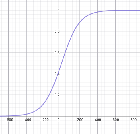
We know the drug design parameter x from the sample, the outcome from patients y have following distribution, y=1 means the drug takes effect :

(4.2.1)p(ฮธ)=p(yi=1|ฮธ)=11+eโˆ’(ฮฒ1+ฮฒ2x)ฮธ=(ฮฒ1,ฮฒ2)D=y

Here ฮฒ1 and ฮฒ2 are unknown drug effect parameters, we know (xi,yi), then the likelihood of one observation is :

(4.2.2)P(yi|ฮธ,xi)=pi(ฮธ)yi[1โˆ’pi(ฮธ)]1โˆ’yi

254

We want to get the posterior probability :

(4.2.3)P(ฮธ|x,y)=P(ฮฒ1,ฮฒ2|xi,yi)

using the Bayes formula, we have :

(4.2.4)P(ฮฒ1,ฮฒ2|y,x)=P(y|ฮฒ1,ฮฒ2,x)P(ฮฒ1)P(ฮฒ2)P(y)=[โˆi=1nP(yi|ฮธ,xi)]ร—P(ฮฒ1)P(ฮฒ2)โˆฌโ€ฆdฮฒ1dฮฒ2

where the first term in nominator comes from (4.2.2). The denominator holds because the ฮฒ1 and ฮฒ2 covers the space. So, in the M-H sampling, we ==don't compute the denominator since it's intractable==. Instead, we set the proposal distribution that prop to the posterior :

(4.2.5)ฯ€~(ฮธ)=P(y|x,ฮธ)P(ฮธ)=โˆi=1n[pi(ฮธ)yi[1โˆ’pi(ฮธ)]1โˆ’yi]ร—P(ฮฒ1)P(ฮฒ2)โˆP(ฮฒ1,ฮฒ2|y)

where ฯ€~ is called unnormalized posterior.

Then use following acceptance computation to sample from posterior distribution :

(4.2.6)ฮฑ(y,x)=min{1,ฯ€~(ฮธnew)ฯ€~(ฮธold)}

5. Gibbs sampling โ€‹

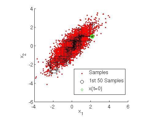
Gibbs sampling is an MCMC method for a multivariate target distribution ฯ€(x1,โ€ฆ,xd) when the full conditional distributions can be sampled.
293

For a two-dimensional target ฯ€(x1,x2), a systematic Gibbs iteration is sample each according to its own distribution ฯ€:

(5.1)X1(t+1)โˆผฯ€(x1โˆฃX2(t)),X2(t+1)โˆผฯ€(x2โˆฃX1(t+1)).

More generally, update one coordinate at a time from its full conditional distribution:

(5.2)Xk(t+1)โˆผฯ€(xkโˆฃX1(t+1),โ€ฆ,Xkโˆ’1(t+1),Xk+1(t),โ€ฆ,Xd(t)).

For example, when x1 is held fixed, moving from (x1,x2) to (x1,x2โ€ฒ) has transition density ฯ€(x2โ€ฒโˆฃx1). The corresponding coordinate-update kernel satisfies

(5.3)ฯ€(x1,x2)ฯ€(x2โ€ฒโˆฃx1)=ฯ€(x1,x2โ€ฒ)ฯ€(x2โˆฃx1),

because ฯ€(x1,x2)=ฯ€(x1)ฯ€(x2โˆฃx1). Consequently, each coordinate-update kernel leaves ฯ€ invariant, and no accept/reject step is required: every Gibbs proposal is accepted.

Systematic versus random scan Each individual coordinate update is reversible. A systematic sequence of coordinate updates still leaves ฯ€ invariant, although the combined full-sweep kernel is not necessarily reversible. Randomly selecting a coordinate at each iteration yields a reversible mixture kernel.

Gibbs sampling can mix slowly when components are strongly correlated, because each move changes only one coordinate. Blocking correlated variables or using more advanced samplers can improve mixing.

References โ€‹

  1. C. P. Robert and G. Casella, Monte Carlo Statistical Methods, 2nd ed., Springer, 2004.
  2. W. R. Gilks, S. Richardson, and D. J. Spiegelhalter (eds.), Markov Chain Monte Carlo in Practice, Chapman & Hall, 1996.
  3. Metropolis-Hastings algorithm (Wikipedia)
  4. Gibbs sampling (Wikipedia)